What is a Neural Network?
By Matthew Viafora

When I first started learning about artificial intelligence and machine learning, I felt that
everything just seemed to work like magic. It was a very overwhelming process to learn about the different algorithms used in the artificial intelligence and machine learning field. Everything seemed like it was behind an unclimbable wall due to the huge mathematical learning curve needed to understand how the algorithms work. One algorithm that seemed to magically draw my curiosity was neural networks. There are many different algorithms involving neural networks that a whole field is dedicated to the advancement of these networks: deep learning. The most interesting aspect that drew me in was the inspiration for neural networks. They were inspired loosely by the structure of a neuron in the brain! This simple idea of the neural network being modeled after the human brain just makes your curiosity run wild with questions of the limits of neural networks and deep learning. Just how much is a neural network able to learn? If it is modeled after the human brain, then wouldn't it be able to learn just about anything? Unfortunately in reality, a neural network does have its limitations and definitely does not involve any kind of magic (unless you count mathematics as magic!). However, neural networks do possess the ability to be applied to many modern day problems which help across a diverse range of industries in the world. By the end of this article, you will be able to understand the structure and function of a basic neural network in machine learning!
Why is it called a neural network? Well, this is because of its inspiration from a neuron in the brain. Each neuron in the human brain has something called Dendrites, which takes in some kind of input, then those inputs are sent through a Myelin sheat (processing) before being pushed to an Axon terminal which is where new information is outputted. A neural network is loosely based on this process as can be seen in the figure below. There can be multiple inputs and multiple outputs of a neural network, just like a brain neuron. The outputs of a neural network are most commonly used for binary classification, however as neural networks become more complex, they are able to classify into multiple output classes, but for now, we will solely focus on binary classification as it is the most basic type of neural network.
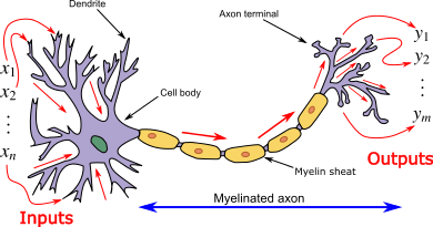
https://en.wikipedia.org/wiki/Artificial_neural_network
Before diving straight into complicated neural networks, it is extremely important to break it down to the basics. Most of the time in machine learning or data science, before administering complicated neural networks/machine learning algorithms, practitioners attempt to solve the problem using a simple algorithm, since most complicated machine learning/deep learning algorithms are derived from the basics. In the case of neural networks, the basic form is simple logistic regression. On a high level, a neural network is just a logistic regression model with more layers. If you do not fully understand logistic regression, that is okay, I will go over how it works! Before looking at the figure below, don’t panic! It may look like a bunch of complicated mathematics, but it is very simple once it is broken down. Note: For brevity, I won’t go deeply into the more complicated parts of logistic regression involving backpropagation. For a more detailed and mathematical explanation, I HIGHLY recommend Andrew Ng’s deep learning course on coursera.
http://datahacker.rs/005-pytorch-logistic-regression-in-pytorch/
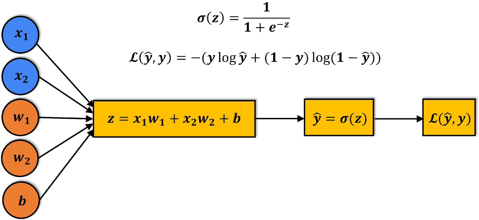
First before we go over what is going on in the figure above, I want you to notice the visual similarities between this figure and the previous one! It follows the same input → processing → output flow as the brain neuron does.
Before going into the process of how logistic regression works, I want to explain the structure of the algorithm. First, as you can see on the left most side of the figure, there are bubbles with some symbols inside of them. The blue bubbles represent the inputs of the logistic regression algorithm, for example this could be the price of a house and the square footage of a house in a model that predicts the probability of whether or not a house will sell. The orange bubbles represent the weights and bias respectively, these will be used during forward and backward propagation to adjust and tweak until the model performs accurately. Note: When describing the logistic regression network, I will refer to the inputs (ex. x1, x2, x3,...,xi) as simply X, and similarly with the weights I will represent them as W. The first box in the figure represents the equation ‘z’ which is the inputs X multiplied by the weights W plus the bias. When calculating weights and biases it is done in the form of matrix multiplication. In this case, X is a matrix of inputs multiplied by a matrix of weights W, to get some matrix of Z values. The next box represents ŷ, which is the value Z ran through what's called an activation function. An activation function, σ, bounds a value between (in this example) 0 and 1. There are different types of activation functions that bound values in different ways, however one of the most commonly used is the sigmoid function (σ) as it bounds a value between 0 and 1. The value obtained by ŷ is equal to the probability of the inputs being correlated to class 0. For example if you were predicting whether a house will sell, you could correlate class 0 to being “will not sell” and class 1 to “will sell”. When making predictions with logistic regression, this is the step where you would get your prediction! There is one more box however farthest to the right. This box represents the loss function L. This function compares ŷ with y where ŷ is the prediction of the model and y is the actual output. The loss function L is used during training to improve the accuracy of the model. Now that we’ve covered the structure of the logistic regression model, let’s dive into how a model is trained!
Logistic regression training works in two parts: forward and backward propagation. Forward propagation is much more straightforward and easier to understand than backward propagation. During forward propagation of logistic regression, the algorithm simply moves forward in the network. First input X is given to the model with weights W and biases B usually randomized (which will most likely give a poor accuracy of the model at first, but that is why we are training it to improve!), from that the model will calculate the z value which we explained above is just X * W + b. The z value will then be fed into the activation function, which in our example is the sigmoid function σ, that bounds the z value between 0 and 1. From this we obtain the value ŷ which is the probability of the inputs X belonging to class 0. Then finally, in forward propagation, we obtain the value of the loss function which compares ŷ to y. This value gives us an understanding of how well the model is performing. This concludes forward propagation in a logistic regression model. What happens next is backward propagation which is a lot more complicated than forward propagation and I often find myself reviewing backward propagation concepts as I am implementing models using logistic regression. Backward propagation involves calculating a series of derivatives to minimize the loss function L. This involves lots of calculus in an algorithm called gradient descent. Below is a visual representation of how gradient descent works to find a minimum of a function.
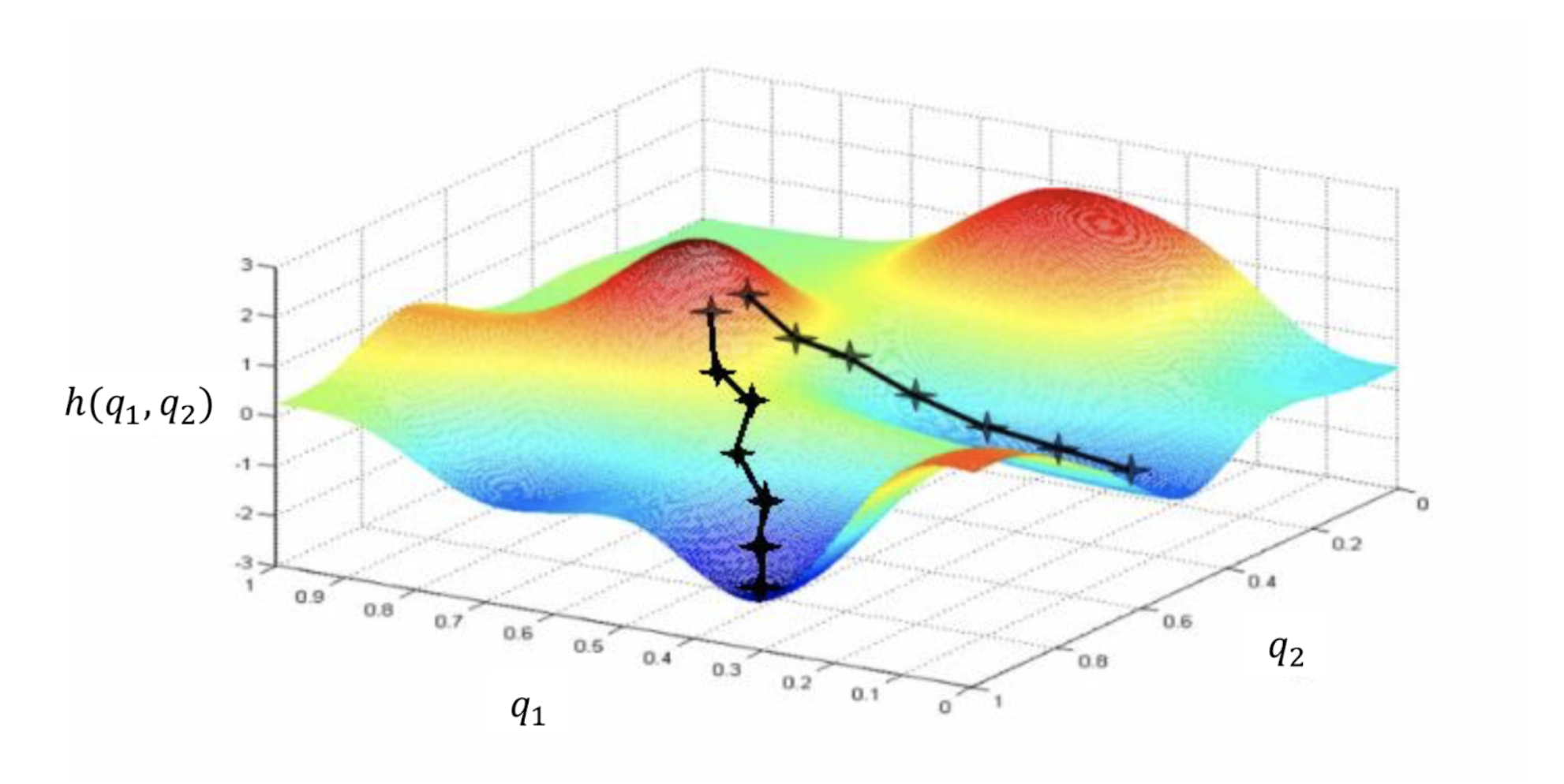
https://shashank-ojha.github.io/ParallelGradientDescent/
In this general figure representing the gradient descent algorithm, you can substitute q1 for ŷ, q2 for y, and the function h(q1, q2) for our loss function L(ŷ, y). As you can see in the figure the goal of gradient descent is to come from a high loss generated from randomly selected weights and bias, and slightly tweak those weights and bias through a series of calculations of derivatives, then move in the direction of the greatest slope downward in order to hopefully find a minimum in the function L. There is lots of mathematics behind this algorithm and it is used heavily in machine learning and other disciplines. I highly recommend doing more research into gradient descent and how it works. It is a very interesting, fun-to-learn, and heavily used algorithm!
During each step of the gradient descent algorithm, the model training is iterating through forward and backward propagation in order to continue tweaking the weights W and biases B in order to improve accuracy and converge the loss function L to a minimum. After the loss function L has converged to a minimum, the training of the algorithm is finished and can be used for predictions!
Now that was a lot of mathematics for just the basics of a neural network, right? Well fortunately, a neural network is simply a logistic regression model with multiple layers. See in the example below! Remember, it is extremely important to understand the basics of logistic regression before moving on to neural networks, so I highly suggest doing more research on how logistic regression works and especially backpropagation and gradient descent.
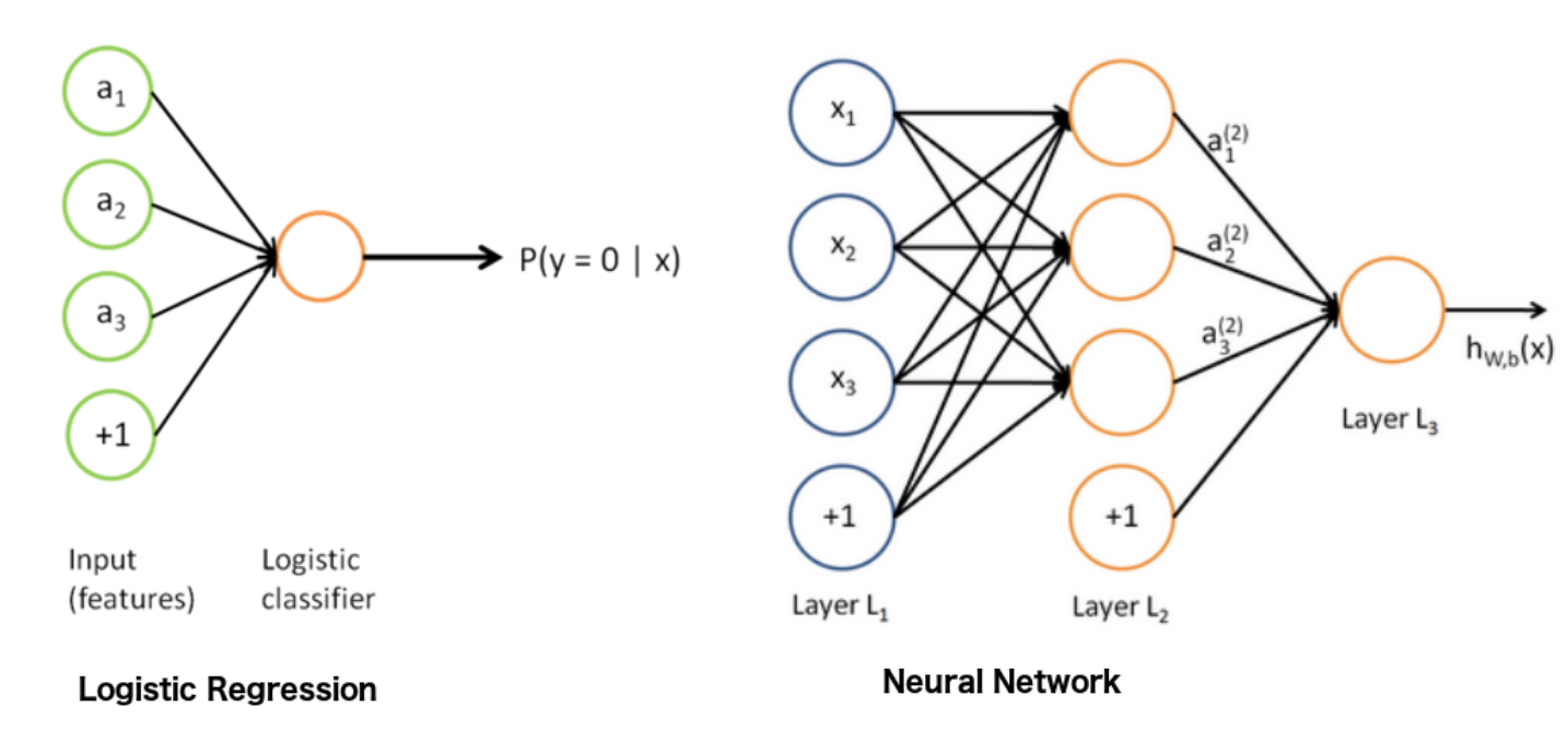
https://stats.stackexchange.com/questions/366707/a-logistic-regression-with-neural-network-mindset-vs-a-shallow-neural-network
As you can see on the left side, we have our familiar logistic regression. (Note: The P(y=0 | x) just means “the probability that y = 0 given x”) Now on the right side we have a neural network, how exciting! As you can see, we have the inputs X given in layer L1 (Note: In this diagram the weights W are considered the lines connecting the layers together and the bias is represented as the node containing “+1”). In the figure above, layer L2 calculates the z value by multiplying the inputs X by the weights W plus the bias B, then runs this z value through an activation function σ giving us ŷ, just like regular old logistic regression! However, in this case, as you can see layer L2 has multiple nodes all calculating different ŷ values. These ŷ outputs of layer L2 will then be used as the inputs X to layer L3, where the layer will do the same calculations that it normally does with logistic regression! Finally, layer L3 will output a ŷ of its own which will be the probability that y = 0. The training of a neural network is almost identical to the training of a logistic regression model just with a few extra layers.
There are many different types of neural network shapes and hyperparameters that a machine learning engineer or data scientist can tune and tweak in order to get the best performing neural network (or logistic regression model!). The tweaking of hyperparameters of a neural network is a complex and tricky topic that I will be sure to save for another article, but whenever you are implementing a neural network or other type of supervised learning model, always remember to try and keep things simple in order to avoid things like overfitting. (Note: I will go over overfitting, underfitting, variance, hyperparameter tuning, etc. in another article, so stay tuned!)
As you can see neural networks are quite literally a multi-layers logistic regression model (Fun fact: another name for a neural network is a “multilayer perceptron”). That is why I emphasize that in order to understand and apply neural networks, it is crucial that one must understand logistic regression completely. In today’s world, there are plenty of libraries and tools that all have the math behind these algorithms built in and all you have to do is apply your training data and predictions. However, I believe that it is important to understand the fundamental underlying math that is taking place in order to create, tune, and maintain the most accurate models possible.
In this article, we went over the fundamentals of logistic regression and neural networks with some visual examples of each. I hope that this article helped introduce you to the intimidating topic of neural networks and deep learning as it is something that I struggled to comprehend when I first started learning about machine learning and deep learning. Be sure to stay tuned for more articles on neural networks and send any feedback that you have to my email found on the “about us” page of this site!
Thank you for reading and keep learning!